Modelos NARX Gerais¶

Exemplo criado por Wilson Rocha Lacerda Junior

Procurando mais detalhes sobre modelos NARMAX? Para informações completas sobre modelos, métodos e uma ampla variedade de exemplos e benchmarks implementados no SysIdentPy, confira nosso livro: Nonlinear System Identification and Forecasting: Theory and Practice With SysIdentPy

Este livro oferece orientação aprofundada para apoiar seu trabalho com o SysIdentPy.

Neste exemplo, criaremos modelos NARX usando diferentes estimadores como GradientBoostingRegressor, Bayesian Regression, Automatic Relevance Determination (ARD) Regression e Catboost.

pip install sysidentpy

import matplotlib.pyplot as plt
from sysidentpy.metrics import mean_squared_error
from sysidentpy.utils.generate_data import get_siso_data
from sysidentpy.general_estimators import NARX
from sklearn.linear_model import BayesianRidge, ARDRegression
from sklearn.ensemble import GradientBoostingRegressor
from catboost import CatBoostRegressor

from sysidentpy.basis_function import Polynomial, Fourier
from sysidentpy.utils.plotting import plot_residues_correlation, plot_results
from sysidentpy.residues.residues_correlation import (
    compute_residues_autocorrelation,
    compute_cross_correlation,
)

# dataset simulado
x_train, x_valid, y_train, y_valid = get_siso_data(
    n=10000, colored_noise=False, sigma=0.01, train_percentage=80
)

Importância da arquitetura NARX¶

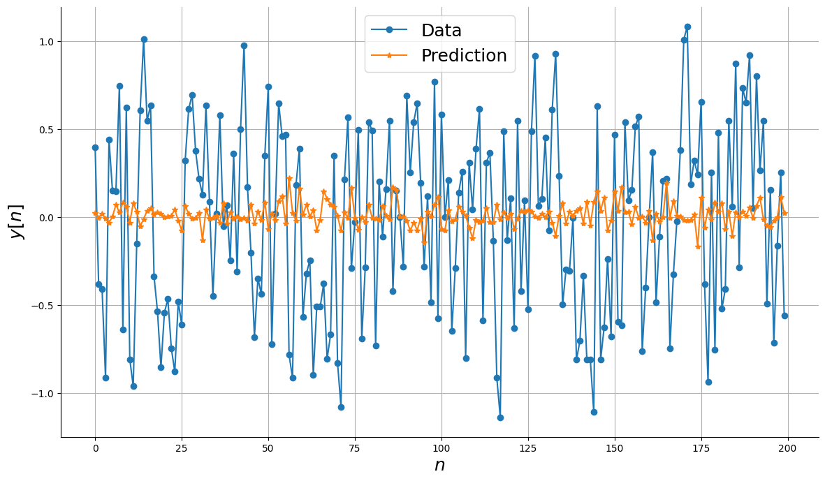
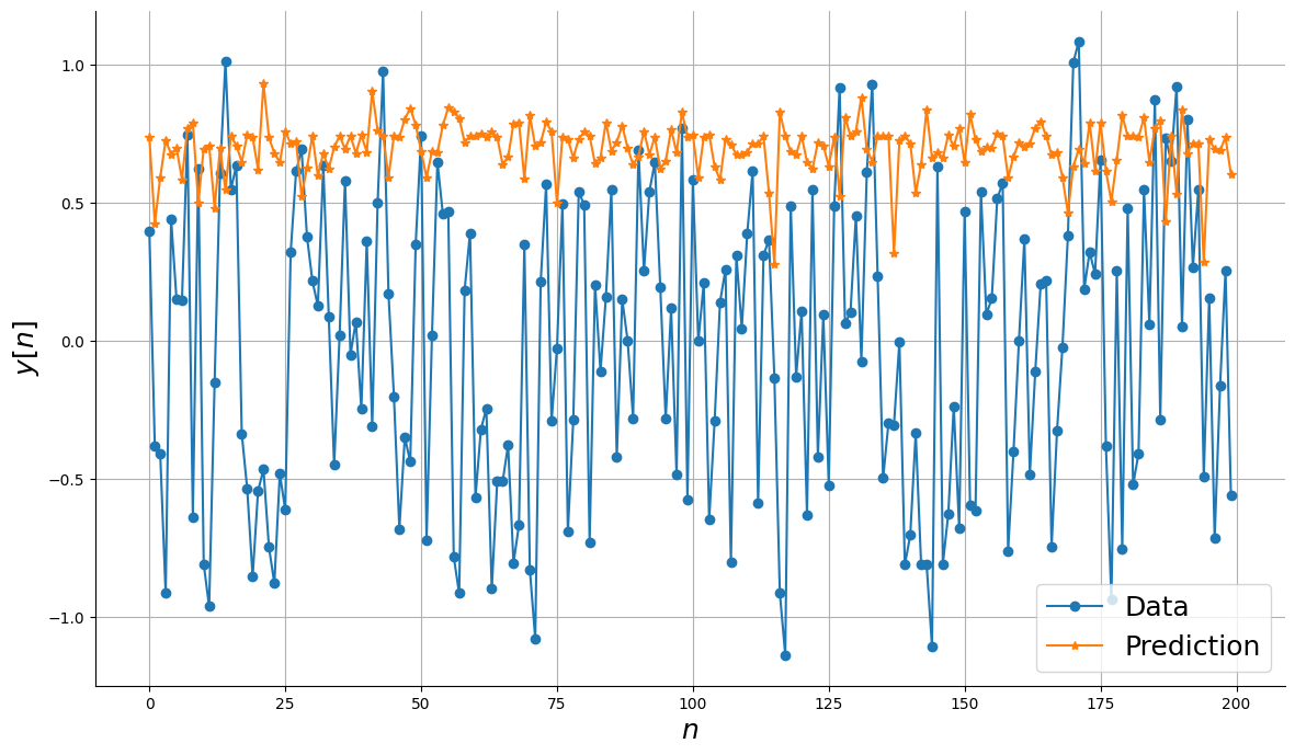
Para ter uma ideia da importância da arquitetura NARX, vamos observar o desempenho dos modelos sem a configuração NARX.

catboost = CatBoostRegressor(iterations=300, learning_rate=0.1, depth=6)

gb = GradientBoostingRegressor(
    loss="quantile",
    alpha=0.90,
    n_estimators=250,
    max_depth=10,
    learning_rate=0.1,
    min_samples_leaf=9,
    min_samples_split=9,
)

def plot_results_tmp(y_valid, yhat):
    _, ax = plt.subplots(figsize=(14, 8))
    ax.plot(y_valid[:200], label="Data", marker="o")
    ax.plot(yhat[:200], label="Prediction", marker="*")
    ax.set_xlabel("$n$", fontsize=18)
    ax.set_ylabel("$y[n]$", fontsize=18)
    ax.grid()
    ax.legend(fontsize=18)
    plt.show()

catboost.fit(x_train, y_train, verbose=False)
plot_results_tmp(y_valid, catboost.predict(x_valid))

gb.fit(x_train, y_train.ravel())
plot_results_tmp(y_valid, gb.predict(x_valid))

Introduzindo a configuração NARX usando SysIdentPy¶

Como você pode ver, basta passar o estimador base desejado para a classe NARX do SysIdentPy para construir o modelo NARX! Você pode escolher os lags das variáveis de entrada e saída para construir a matriz de regressores.

Mantemos o método fit/predict para tornar o processo direto.

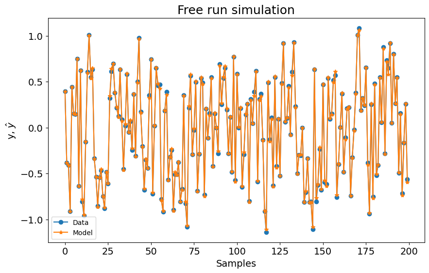
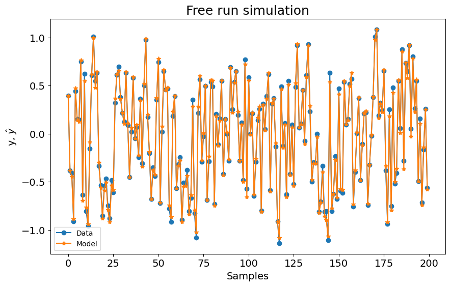
NARX com Catboost¶

basis_function = Fourier(degree=1)

catboost_narx = NARX(
    base_estimator=CatBoostRegressor(iterations=300, learning_rate=0.1, depth=8),
    xlag=10,
    ylag=10,
    basis_function=basis_function,
    model_type="NARMAX",
    fit_params={"verbose": False},
)

catboost_narx.fit(X=x_train, y=y_train)
yhat = catboost_narx.predict(X=x_valid, y=y_valid, steps_ahead=1)
print("MSE: ", mean_squared_error(y_valid, yhat))
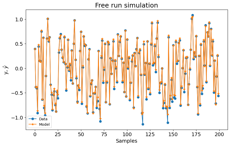
plot_results(y=y_valid, yhat=yhat, n=200)
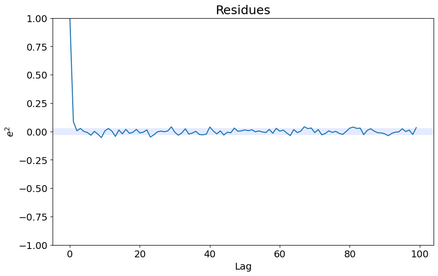
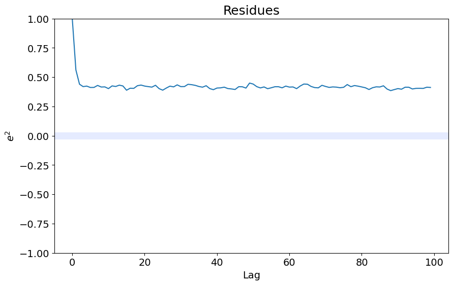
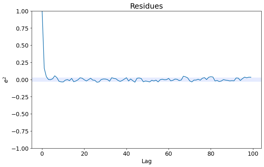
ee = compute_residues_autocorrelation(y_valid, yhat)
plot_residues_correlation(data=ee, title="Residues", ylabel="$e^2$")
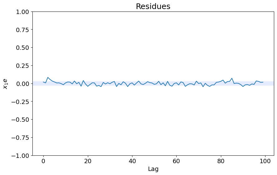
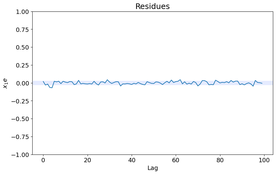
x1e = compute_cross_correlation(y_valid, yhat, x_valid)
plot_residues_correlation(data=x1e, title="Residues", ylabel="$x_1e$")

MSE:  0.00024145290395678653

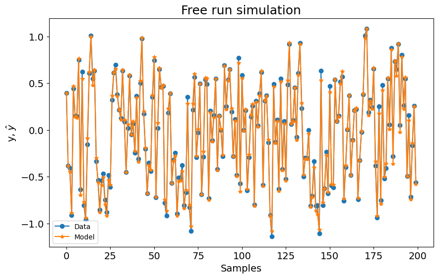
NARX com Gradient Boosting¶

basis_function = Fourier(degree=1)

gb_narx = NARX(
    base_estimator=GradientBoostingRegressor(
        loss="quantile",
        alpha=0.90,
        n_estimators=250,
        max_depth=10,
        learning_rate=0.1,
        min_samples_leaf=9,
        min_samples_split=9,
    ),
    xlag=2,
    ylag=2,
    basis_function=basis_function,
    model_type="NARMAX",
)

gb_narx.fit(X=x_train, y=y_train)
yhat = gb_narx.predict(X=x_valid, y=y_valid)
print(mean_squared_error(y_valid, yhat))

plot_results(y=y_valid, yhat=yhat, n=200)
ee = compute_residues_autocorrelation(y_valid, yhat)
plot_residues_correlation(data=ee, title="Residues", ylabel="$e^2$")
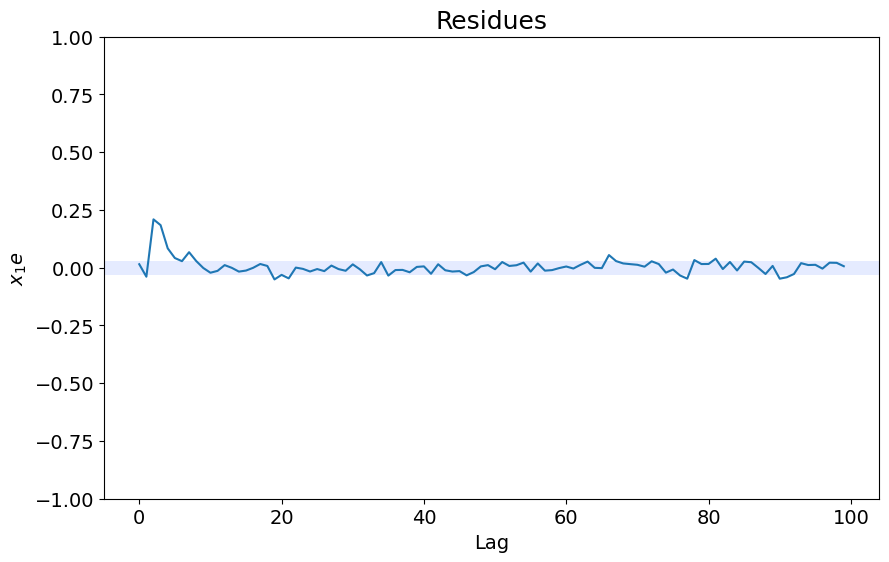
x1e = compute_cross_correlation(y_valid, yhat, x_valid)
plot_residues_correlation(data=x1e, title="Residues", ylabel="$x_1e$")

0.0011824693986863938

NARX com ARD¶

from sysidentpy.general_estimators import NARX

ARD_narx = NARX(
    base_estimator=ARDRegression(),
    xlag=2,
    ylag=2,
    basis_function=basis_function,
    model_type="NARMAX",
)

ARD_narx.fit(X=x_train, y=y_train)
yhat = ARD_narx.predict(X=x_valid, y=y_valid)
print(mean_squared_error(y_valid, yhat))

plot_results(y=y_valid, yhat=yhat, n=200)
ee = compute_residues_autocorrelation(y_valid, yhat)
plot_residues_correlation(data=ee, title="Residues", ylabel="$e^2$")
x1e = compute_cross_correlation(y_valid, yhat, x_valid)
plot_residues_correlation(data=x1e, title="Residues", ylabel="$x_1e$")

0.0011058934497373794

NARX com Bayesian Ridge¶

from sysidentpy.general_estimators import NARX

BayesianRidge_narx = NARX(
    base_estimator=BayesianRidge(),
    xlag=2,
    ylag=2,
    basis_function=basis_function,
    model_type="NARMAX",
)

BayesianRidge_narx.fit(X=x_train, y=y_train)
yhat = BayesianRidge_narx.predict(X=x_valid, y=y_valid)
print(mean_squared_error(y_valid, yhat))

plot_results(y=y_valid, yhat=yhat, n=200)
ee = compute_residues_autocorrelation(y_valid, yhat)
plot_residues_correlation(data=ee, title="Residues", ylabel="$e^2$")
x1e = compute_cross_correlation(y_valid, yhat, x_valid)
plot_residues_correlation(data=x1e, title="Residues", ylabel="$x_1e$")

0.0011077874945734536

Nota¶

Lembre-se que você pode usar predição n-steps-ahead e modelos NAR e NFIR agora. Confira como usá-los em seus respectivos exemplos.