Electromechanical System Identification - MetaMSS¶

Example created by Wilson Rocha Lacerda Junior

Looking for more details on NARMAX models? For comprehensive information on models, methods, and a wide range of examples and benchmarks implemented in SysIdentPy, check out our book: Nonlinear System Identification and Forecasting: Theory and Practice With SysIdentPy

This book provides in-depth guidance to support your work with SysIdentPy.

import pandas as pd
import numpy as np
import matplotlib.pyplot as plt
from sklearn.preprocessing import StandardScaler
from sysidentpy.model_structure_selection import MetaMSS, FROLS
from sysidentpy.metrics import root_relative_squared_error
from sysidentpy.basis_function import Polynomial
from sysidentpy.parameter_estimation import RecursiveLeastSquares
from sysidentpy.utils.display_results import results
from sysidentpy.utils.plotting import plot_residues_correlation, plot_results
from sysidentpy.residues.residues_correlation import (
    compute_residues_autocorrelation,
    compute_cross_correlation,
)

data_url = (
    "https://raw.githubusercontent.com/wilsonrljr/sysidentpy-data/"
    "4085901293ba5ed5674bb2911ef4d1fa20f3438d/datasets/generator/"
)
df1 = pd.read_csv(f"{data_url}x_cc.csv", header=None)
df2 = pd.read_csv(f"{data_url}y_cc.csv", header=None)

df2[5000:80000].plot(figsize=(10, 4))

<Axes: >

df1.iloc[::500].values.shape

(1000, 1)

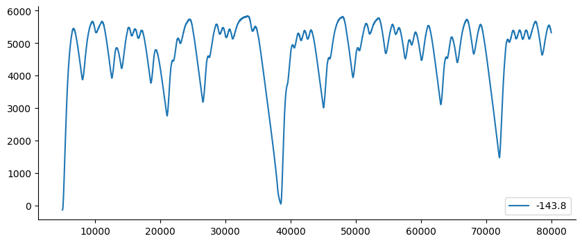
We decimate the data using \(d=500\) and split the resulting 1,000 samples into equal identification and validation sets. Input and output standardization is fitted only on the identification set; the fitted transformations are then applied to validation data, preventing information leakage.

# We decimate the data using d=500 in this example.
x_train, x_test = np.split(df1.iloc[::500].values, 2)
y_train, y_test = np.split(df2.iloc[::500].values, 2)

x_scaler = StandardScaler()
y_scaler = StandardScaler()
x_train_scaled = x_scaler.fit_transform(x_train)
x_test_scaled = x_scaler.transform(x_test)
y_train_scaled = y_scaler.fit_transform(y_train)
y_test_scaled = y_scaler.transform(y_test)

basis_function = Polynomial(degree=2)
estimator = RecursiveLeastSquares(lam=0.95, delta=0.01)

model = MetaMSS(
    xlag=5,
    ylag=5,
    estimator=estimator,
    maxiter=5,
    n_agents=15,
    basis_function=basis_function,
    random_state=42,
)

with np.errstate(over="ignore", invalid="ignore", divide="ignore"):
    model.fit(X=x_train_scaled, y=y_train_scaled)

The search may evaluate candidates whose recursions are numerically invalid. np.errstate suppresses only those expected numerical warnings; predictions from the selected model are explicitly checked before evaluation.

yhat_free_scaled = model.predict(
    X=x_test_scaled, y=y_test_scaled, steps_ahead=None
)
yhat_one_step_scaled = model.predict(
    X=x_test_scaled, y=y_test_scaled, steps_ahead=1
)

yhat_free = y_scaler.inverse_transform(yhat_free_scaled)
yhat_one_step = y_scaler.inverse_transform(yhat_one_step_scaled)

if not (np.isfinite(yhat_free).all() and np.isfinite(yhat_one_step).all()):
    raise RuntimeError("The selected model produced a non-finite prediction.")

start = model.max_lag
y_eval = y_test[start:]
yhat_free_eval = yhat_free[start:]
yhat_one_step_eval = yhat_one_step[start:]
x_eval = x_test[start:]

rrse_free = root_relative_squared_error(y_eval, yhat_free_eval)
rrse_one_step = root_relative_squared_error(y_eval, yhat_one_step_eval)
print(f"Free-run RRSE: {rrse_free:.6f}")
print(f"One-step-ahead RRSE: {rrse_one_step:.6f}")

r = pd.DataFrame(
    results(
        model.final_model,
        model.theta,
        model.err,
        model.n_terms,
        err_precision=8,
        dtype="sci",
    ),
    columns=["Regressors", "Parameters", "ERR"],
)
print(r)

plot_results(
    y=y_eval,
    yhat=yhat_free_eval,
    n=1000,
    title=f"Free run simulation — RRSE {rrse_free:.6f}",
)
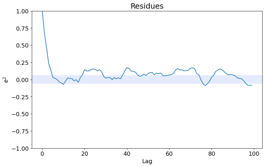
ee = compute_residues_autocorrelation(y_eval, yhat_free_eval)
plot_residues_correlation(data=ee, title="Residues", ylabel="$e^2$")
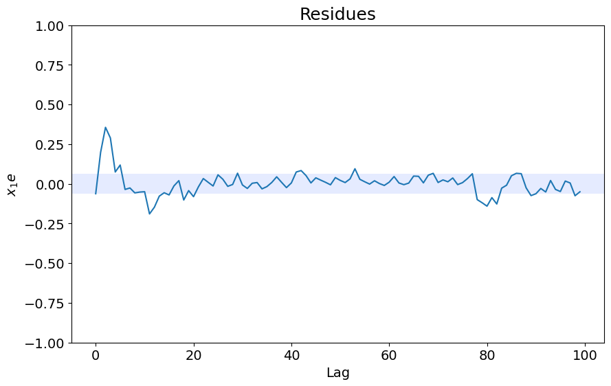
x1e = compute_cross_correlation(y_eval, yhat_free_eval, x_eval)
plot_residues_correlation(data=x1e, title="Residues", ylabel="$x_1e$")

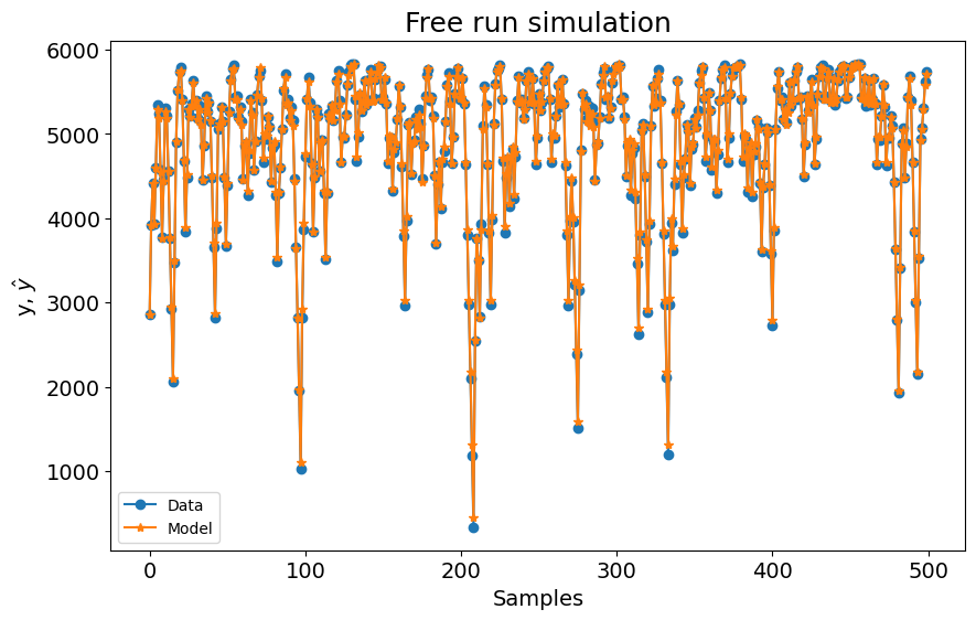
Free-run RRSE: 0.031354
One-step-ahead RRSE: 0.022595
        Regressors   Parameters             ERR
0           y(k-1)   7.0968E-01  0.00000000E+00
1           y(k-3)  -5.8259E-02  0.00000000E+00
2           y(k-4)  -1.0981E-04  0.00000000E+00
3          x1(k-1)   3.7458E-01  0.00000000E+00
4          x1(k-4)   2.2133E-01  0.00000000E+00
5         y(k-1)^2  -2.2259E-02  0.00000000E+00
6     y(k-2)y(k-1)   1.3530E-02  0.00000000E+00
7     y(k-3)y(k-1)   1.6170E-02  0.00000000E+00
8     y(k-4)y(k-1)  -2.0950E-02  0.00000000E+00
9     y(k-5)y(k-1)  -5.9322E-03  0.00000000E+00
10   x1(k-1)y(k-1)  -4.1207E-01  0.00000000E+00
11   x1(k-2)y(k-1)  -1.6460E-01  0.00000000E+00
12    y(k-4)y(k-2)   1.0074E-02  0.00000000E+00
13    y(k-5)y(k-2)   1.4187E-02  0.00000000E+00
14   x1(k-1)y(k-2)   2.8701E-01  0.00000000E+00
15   x1(k-3)y(k-2)   3.5765E-03  0.00000000E+00
16        y(k-3)^2  -1.2085E-02  0.00000000E+00
17    y(k-4)y(k-3)   8.3141E-03  0.00000000E+00
18   x1(k-1)y(k-3)  -1.2719E-01  0.00000000E+00
19   x1(k-2)y(k-3)   2.9013E-02  0.00000000E+00
20   x1(k-4)y(k-3)   9.3360E-03  0.00000000E+00
21   x1(k-1)y(k-4)   3.6354E-02  0.00000000E+00
22        y(k-5)^2  -3.4384E-03  0.00000000E+00
23   x1(k-1)y(k-5)  -1.3772E-03  0.00000000E+00
24   x1(k-5)y(k-5)  -1.0137E-03  0.00000000E+00
25  x1(k-2)x1(k-1)  -1.1732E-02  0.00000000E+00
26  x1(k-5)x1(k-1)   6.8615E-03  0.00000000E+00
27       x1(k-2)^2   1.8984E+00  0.00000000E+00
28  x1(k-3)x1(k-2)  -8.0513E-03  0.00000000E+00
29  x1(k-5)x1(k-2)  -2.0967E-03  0.00000000E+00
30       x1(k-4)^2  -1.8366E+00  0.00000000E+00
31       x1(k-5)^2  -8.7361E-03  0.00000000E+00

With the same data split, lags, polynomial basis, search budget and seed, the effect of standardization and the RLS forgetting factor is compactly summarized as follows:

Data treatment	`lam`	Free-run RRSE	One-step-ahead RRSE
Without standardization	0.98	2.184406	0.037653
Standardized	0.98	0.035944	0.021008
Standardized	0.95	0.031354	0.022595

The code above uses the last configuration. Both prediction modes are generated in standardized coordinates, transformed back to the original output scale and evaluated only after model.max_lag. The comparison shows that preprocessing and the prediction mode are both essential parts of the reported result.

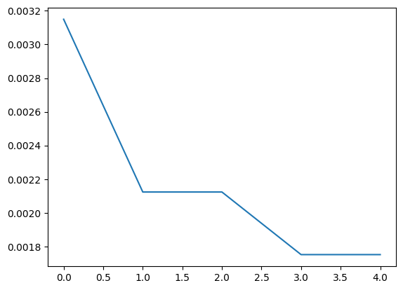
# Plotting the evolution of the agents
plt.plot(model.best_by_iter, marker="o")
plt.title("Optimization evolution")
plt.xlabel("Iteration")
plt.ylabel("Best MetaMSS loss")
model.best_by_iter[-1]

0.0019710527

# You have access to all tested models
# model.tested_models

from sklearn.neighbors import KNeighborsRegressor
from sklearn.tree import DecisionTreeRegressor
from sklearn.ensemble import RandomForestRegressor
from catboost import CatBoostRegressor
from sklearn.linear_model import ARDRegression
from sysidentpy.general_estimators import NARX

xlag = ylag = 5

estimators = [
    (
        "NARX_KNeighborsRegressor",
        NARX(
            base_estimator=KNeighborsRegressor(),
            xlag=xlag,
            ylag=ylag,
            basis_function=basis_function,
        ),
    ),
    (
        "NARX_DecisionTreeRegressor",
        NARX(
            base_estimator=DecisionTreeRegressor(random_state=42),
            xlag=xlag,
            ylag=ylag,
            basis_function=basis_function,
        ),
    ),
    (
        "NARX_RandomForestRegressor",
        NARX(
            base_estimator=RandomForestRegressor(
                n_estimators=200, random_state=42
            ),
            xlag=xlag,
            ylag=ylag,
            basis_function=basis_function,
        ),
    ),
    (
        "NARX_Catboost",
        NARX(
            base_estimator=CatBoostRegressor(
                iterations=800,
                learning_rate=0.1,
                depth=8,
                random_seed=42,
                allow_writing_files=False,
            ),
            xlag=xlag,
            ylag=ylag,
            basis_function=basis_function,
            fit_params={"verbose": False},
        ),
    ),
    (
        "NARX_ARD",
        NARX(
            base_estimator=ARDRegression(),
            xlag=xlag,
            ylag=ylag,
            basis_function=basis_function,
        ),
    ),
    (
        "FROLS-Polynomial_NARX",
        FROLS(
            order_selection=True,
            n_info_values=50,
            ylag=ylag,
            xlag=xlag,
            basis_function=basis_function,
            info_criteria="bic",
            err_tol=None,
        ),
    ),
    (
        "MetaMSS",
        MetaMSS(
            norm=-2,
            xlag=xlag,
            ylag=ylag,
            estimator=estimator,
            maxiter=5,
            n_agents=15,
            loss_func="metamss_loss",
            basis_function=basis_function,
            random_state=42,
        ),
    ),
]


all_results = {}
for model_name, modelo in estimators:
    all_results["%s" % model_name] = []
    with np.errstate(over="ignore", invalid="ignore", divide="ignore"):
        modelo.fit(X=x_train_scaled, y=y_train_scaled)
    yhat_scaled = modelo.predict(X=x_test_scaled, y=y_test_scaled)
    yhat = y_scaler.inverse_transform(yhat_scaled)
    start = modelo.max_lag
    result = root_relative_squared_error(y_test[start:], yhat[start:])
    all_results["%s" % model_name].append(result)
    print(model_name, "%.3f" % np.mean(result))

NARX_KNeighborsRegressor 0.166
NARX_DecisionTreeRegressor 0.413
NARX_RandomForestRegressor 0.263
NARX_Catboost 0.104
NARX_ARD 0.074
FROLS-Polynomial_NARX 0.080
MetaMSS 0.031

for model_name, metric in sorted(
    all_results.items(), key=lambda x: np.mean(x[1]), reverse=False
):
    print(model_name, np.mean(metric))

MetaMSS 0.0313536683
NARX_ARD 0.0739274875
FROLS-Polynomial_NARX 0.0802556552
NARX_Catboost 0.1040535249
NARX_KNeighborsRegressor 0.1658751918
NARX_RandomForestRegressor 0.2629589141
NARX_DecisionTreeRegressor 0.4132172020