Simulate Existing Models
Example created by Wilson Rocha Lacerda Junior
Looking for more details on NARMAX models? For comprehensive information on models, methods, and a wide range of examples and benchmarks implemented in SysIdentPy, check out our book: Nonlinear System Identification and Forecasting: Theory and Practice With SysIdentPy
This book provides in-depth guidance to support your work with SysIdentPy.
import numpy as np
import pandas as pd
from sysidentpy.simulation import SimulateNARMAX
from sysidentpy.metrics import root_relative_squared_error
from sysidentpy.utils.generate_data import get_siso_data
from sysidentpy.basis_function import Polynomial
from sysidentpy.parameter_estimation import LeastSquares
from sysidentpy.utils.display_results import results
from sysidentpy.utils.plotting import plot_residues_correlation, plot_results
from sysidentpy.residues.residues_correlation import (
    compute_residues_autocorrelation,
    compute_cross_correlation,
)
Generating 1 input 1 output sample data
The data is generated by simulating the following model:
\(y_k = 0.2y_{k-1} + 0.1y_{k-1}x_{k-1} + 0.9x_{k-2} + e_{k}\)
If colored_noise is set to True:
\(e_{k} = 0.8\nu_{k-1} + \nu_{k}\)
where \(x\) is a uniformly distributed random variable and \(\nu\) is a gaussian distributed variable with \(\mu=0\) and \(\sigma=0.1\)
In the next example we will generate a data with 1000 samples with white noise and selecting 90% of the data to train the model.
np.random.seed(42)

x_train, x_test, y_train, y_test = get_siso_data(
    n=1000, colored_noise=False, sigma=0.001, train_percentage=90
)
Defining the model
We already know that the generated data is a result of the model \(𝑦_𝑘=0.2𝑦_{𝑘−1}+0.1𝑦_{𝑘−1}𝑥_{𝑘−1}+0.9𝑥_{𝑘−2}+𝑒_𝑘\) . Thus, we can create a model with those regressors follwing a codification pattern: - \(0\) is the constant term, - \([1001] = y_{k-1}\) - \([100n] = y_{k-n}\) - \([200n] = x1_{k-n}\) - \([300n] = x2_{k-n}\) - \([1011, 1001] = y_{k-11} \times y_{k-1}\) - \([100n, 100m] = y_{k-n} \times y_{k-m}\) - \([12001, 1003, 1001] = x11_{k-1} \times y_{k-3} \times y_{k-1}\) - and so on
Important Note
The order of the codes within each model row matters.
If you use [2001, 1001], it will work, but [1001, 2001] will not (the regressor will be ignored). Always put the highest value first: - \([2003, 2001]\) works - \([2001, 2003]\) do not work
We will handle this limitation in an upcoming update. The model rows may be listed in any order, but each value in theta must correspond to the model row at the same position.
s = SimulateNARMAX(
    basis_function=Polynomial(), calculate_err=True, estimate_parameter=False
)

# the model must be a numpy array
model = np.array(
    [
        [1001, 0],  # y(k-1)
        [2001, 1001],  # x1(k-1)y(k-1)
        [2002, 0],  # x1(k-2)
    ]
)
# theta must have shape (n, 1) and follow the row order of model
theta = np.array([[0.2, 0.1, 0.9]]).T
Simulating the model
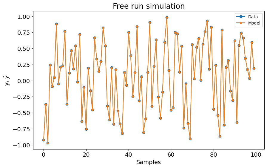
After defining the model and theta we just need to use the simulate method.
The simulate method returns the predicted values and the results where we can look at regressors, parameters and ERR values.
yhat = s.simulate(
    X_test=x_test,
    y_test=y_test,
    model_code=model,
    theta=theta,
)

r = pd.DataFrame(
    results(s.final_model, s.theta, s.err, s.n_terms, err_precision=8, dtype="sci"),
    columns=["Regressors", "Parameters", "ERR"],
)
print(r)

plot_results(y=y_test, yhat=yhat, n=1000)
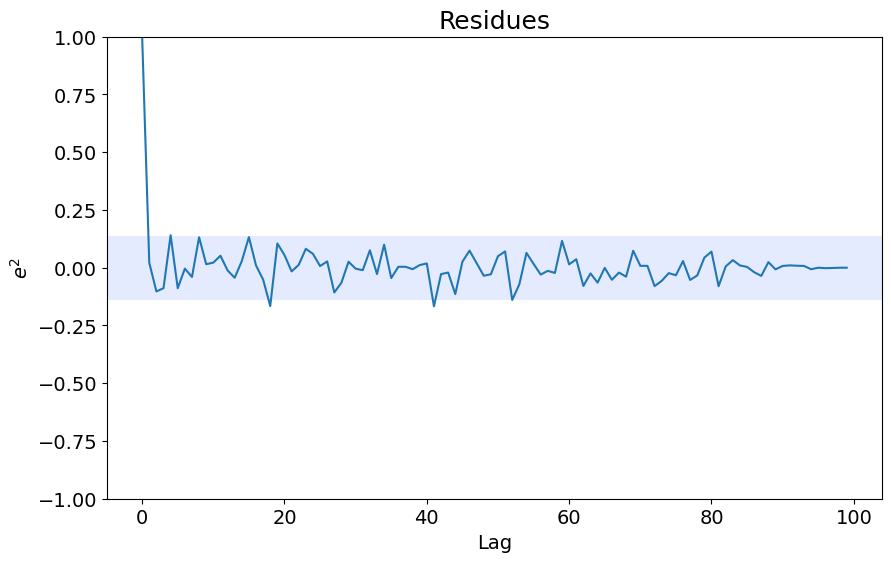
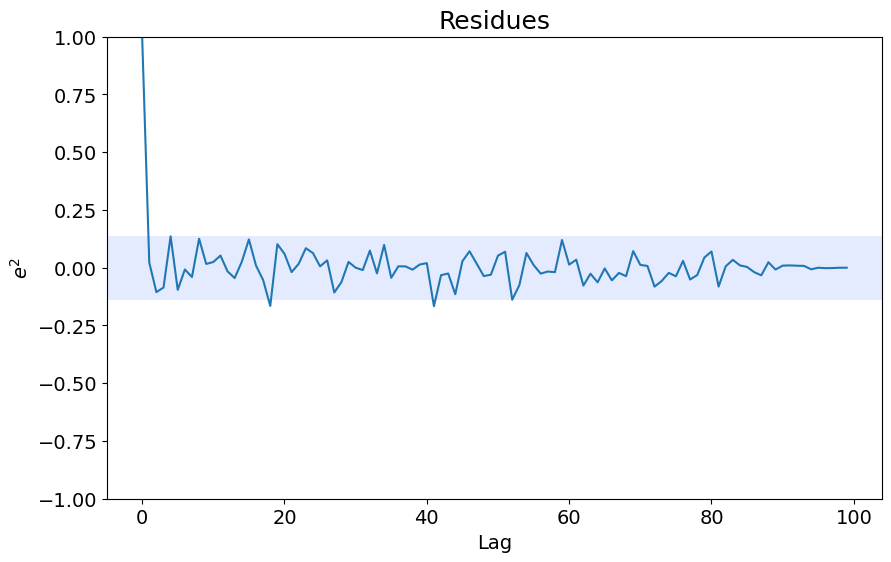
ee = compute_residues_autocorrelation(y_test, yhat)
plot_residues_correlation(data=ee, title="Residues", ylabel="$e^2$")
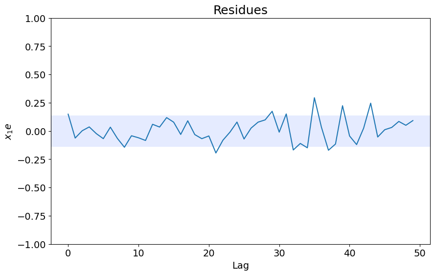
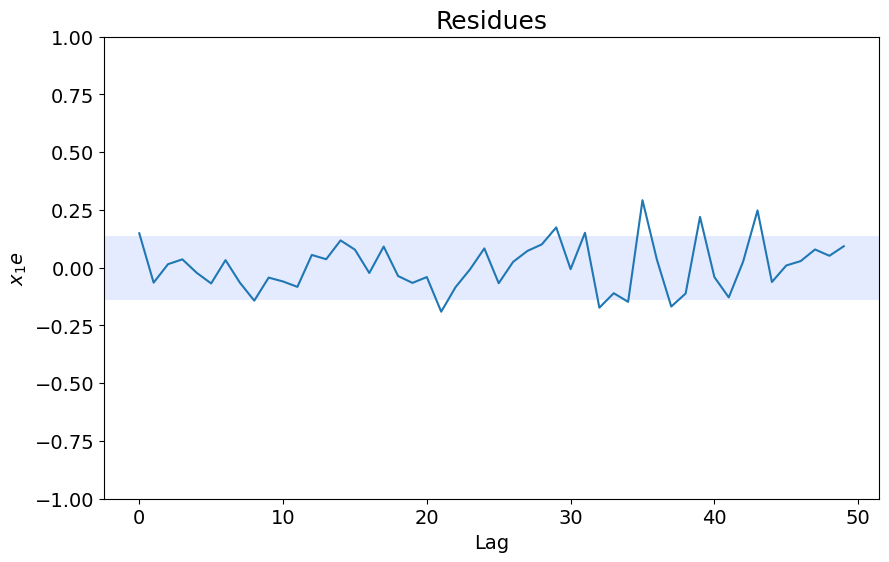
x1e = compute_cross_correlation(y_test, yhat, x_test)
plot_residues_correlation(data=x1e, title="Residues", ylabel="$x_1e$")
      Regressors  Parameters             ERR
0         y(k-1)  2.0000E-01  0.00000000E+00
1  x1(k-1)y(k-1)  1.0000E-01  0.00000000E+00
2        x1(k-2)  9.0000E-01  0.00000000E+00
Options
You can set the steps_ahead to run the prediction/simulation:
yhat = s.simulate(
    X_test=x_test,
    y_test=y_test,
    model_code=model,
    theta=theta,
    steps_ahead=1,
)
rrse = root_relative_squared_error(y_test, yhat)
print(rrse)
0.0018437406169225401
yhat = s.simulate(
    X_test=x_test,
    y_test=y_test,
    model_code=model,
    theta=theta,
    steps_ahead=21,
)
rrse = root_relative_squared_error(y_test, yhat)
print(rrse)
0.0018771888780714843
Estimating the parameters
If you have only the model strucuture, you can create an object with estimate_parameter=True and choose the methed for estimation using estimator. In this case, you have to pass the training data for parameters estimation.
When estimate_parameter=True, we also computate the ERR considering only the regressors defined by the user.
s = SimulateNARMAX(
    basis_function=Polynomial(),
    estimate_parameter=True,
    estimator=LeastSquares(),
    calculate_err=True,
)

yhat = s.simulate(
    X_train=x_train,
    y_train=y_train,
    X_test=x_test,
    y_test=y_test,
    model_code=model,
    # theta will be estimated using the defined estimator
)

r = pd.DataFrame(
    results(s.final_model, s.theta, s.err, s.n_terms, err_precision=8, dtype="sci"),
    columns=["Regressors", "Parameters", "ERR"],
)
print(r)

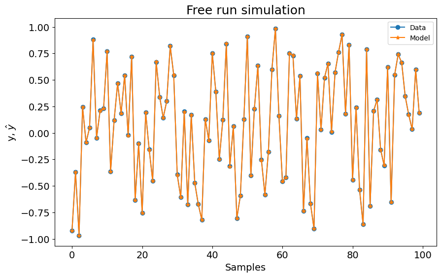
plot_results(y=y_test, yhat=yhat, n=1000)
ee = compute_residues_autocorrelation(y_test, yhat)
plot_residues_correlation(data=ee, title="Residues", ylabel="$e^2$")
x1e = compute_cross_correlation(y_test, yhat, x_test)
plot_residues_correlation(data=x1e, title="Residues", ylabel="$x_1e$")
      Regressors  Parameters             ERR
0         y(k-1)  2.0002E-01  9.55432286E-01
1  x1(k-1)y(k-1)  1.0004E-01  4.12434401E-02
2        x1(k-2)  8.9998E-01  3.32077000E-03